Circuits
In Strawberry Fields, photonic quantum circuits are represented as Program
objects. By creating a program, quantum operations can be applied, measurements performed,
and the program can then be simulated using the various Strawberry Fields backends.
See also
New to photonic quantum computing? See the Glossary for a glossary of some of the terms used in Strawberry Fields.
Creating a quantum program
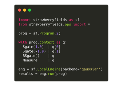
To construct a photonic quantum circuit in Strawberry Fields, a Program object
must be created, and operations applied.
import strawberryfields as sf
from strawberryfields import ops

# create a 3-mode quantum program
prog = sf.Program(3)

with prog.context as q:
    ops.Sgate(0.54) | q[0]
    ops.Sgate(0.54) | q[1]
    ops.Sgate(0.54) | q[2]
    ops.BSgate(0.43, 0.1) | (q[0], q[2])
    ops.BSgate(0.43, 0.1) | (q[1], q[2])
    ops.MeasureFock() | q
Here, we are creating a 3-mode program, and applying a Sgate and
a BSgate to various modes. Constructing quantum circuits always follows
the same structure as the above example; in particular,
A
withstatement is used to populate the program with quantum operations.Program.contextis used within thewithstatement to returnq, a representation of the quantum registers (qumodes or modes).Quantum operations are applied to the modes of the program using the syntax
ops.GateName(arg1, arg2) | (q[i], q[j], ...)
where
ops.GateNameis a quantum operation,arg1, arg2are its parameters, and the right-hand side of the vertical bar lists the qumode(s) on which the operation will act.
Note
The contents of a program can be viewed by calling the Program.print() method,
or output as a qcircuit \(\LaTeX{}\) document by using the Program.draw_circuit()
method.
See also
Visit the Operations page to see an overview of available quantum operations.
See also
Strawberry Fields also provides support for constructing and simulating photonic
time domain multiplexing algorithms. For more details, please see TDMProgram.
Simulating your program
Strawberry Fields provides several backend simulators for simulating your quantum program. To access the simulators, an engine must be initialized, which is responsible for executing the program on a specified backend (which can be either a local simulator, or a remote simulator/hardware device).
# initialize the fock backend with a
# Fock cutoff dimension (truncation) of 5
eng = sf.Engine("fock", backend_options={"cutoff_dim": 5})
Engine accepts two arguments, the backend name, and a dictionary of
backend options. Available backends include:
The
'fock'backend, written in NumPy.This backend represents the quantum state and operations via the Fock basis, so can represent all possible CV states and operations. However numerical error is also introduced due to truncation of the Fock space—increasing the cutoff results in higher accuracy at a cost of increased memory consumption.
The
'gaussian'backend, written in NumPy.This backend represents the quantum state as a Gaussian, and operations as quantum operations. It is numerically exact, and consumes less memory and is less computationally intensive then the Fock backends. However, it cannot represent non-Gaussian operations and states, with the exception of terminal Fock measurements.
The
'bosonic'backend, written in NumPy.The bosonic backend is tailored to simulate states which can be represented as a linear combination of Gaussian functions in phase space. It provides very succinct descriptions of Gaussian states, just like the
gaussianbackend, but it can also provide descriptions of non-Gaussian states as well. Moreover, like in the gaussian backend, the application of the most common active and passive linear optical operations, like the displacement (Dgate, squeezing (Sgate), and beamsplitter (BSgate) gates, is extremely efficient.The
'tf'backend, written in TensorFlow 2.This backend represents the quantum state and operations via the Fock basis, but allows for backpropagation and optimization using TensorFlow.
Note
To instantiate an engine with the TensorFlow backend, TensorFlow 2.0 and above must be installed. In most cases, TensorFlow can be installed via
pip:pip install tensorflowFor more installation details and instructions, please refer to the TensorFlow documentation.
Once the engine has been initialized, the quantum program can be executed on the
selected backend via Engine.run():
result = eng.run(prog)
Execution results
The returned Result object provides several useful properties
for accessing the results of your program execution:
Result.state: The quantum state object contains details and methods for manipulation of the final circuit state. Not available for remote backends.>>> print(result.state) <FockState: num_modes=3, cutoff=5, pure=True, hbar=2.0> >>> state = result.state >>> state.trace() # trace of the quantum state 0.9999999999999999 >>> state.dm().shape # density matrix (5, 5, 5, 5, 5, 5)
Result.samples: Measurement samples from any measurements performed.>>> results.samples [0, 0, 2]
See also
Visit the States page to see an overview of available quantum state methods.
Note
Measured modes will always be returned to the vacuum state.
Warning
To avoid significant numerical error when working with Fock backends, ensure that
the trace of your program after simulation remains reasonably close to 1,
by calling state.trace(). If the trace is much less than 1, you
will need to increase the cutoff dimension.
Symbolic parameters
The quantum operations can take both numerical and symbolic parameters. The latter fall into two types:
Measured parameters: Certain quantum programs (e.g. quantum teleportation) require that operations can be conditioned on measurement results obtained during the execution of the program. In this case the parameter value is not known until the measurement is made (or simulated). The latest measurement result of qumode
iis available viaq[i].par.Free parameters: A parametrized circuit template is a program that depends on a number of free parameters. These parameters can be bound to new fixed values each time the program is executed. The free parameters are created and accessed using the
Program.params()method.
The symbolic parameters can be combined and transformed using basic algebraic operations, and
the mathematical functions in the strawberryfields.math namespace.
import strawberryfields as sf
from strawberryfields import ops

# create a 2-mode quantum program
prog = sf.Program(2)

# create a free parameter named 'a'
a = prog.params('a')

# define the program
with prog.context as q:
    ops.Dgate(a ** 2)    | q[0]  # free parameter
    ops.MeasureX         | q[0]  # measure qumode 0, the result is used in the next operation
    ops.Sgate(1 - sf.math.sin(q[0].par)) | q[1]  # measured parameter
    ops.MeasureFock()    | q[1]

# initialize the Fock backend
eng = sf.Engine('fock', backend_options={'cutoff_dim': 5})

# run the program, with the free parameter 'a' bound to the value 0.9
result = eng.run(prog, args={'a': 0.9})
Warning
When using the TensorFlow backend, all Tensor and Variable objects must be passed to gates by using a free parameter, and binding the Tensor/Variable on engine execution. For more details, see Optimization & machine learning with TensorFlow.
Compilation
The Program object also provides the Program.compile() method that
automatically transforms your circuit into an equivalent circuit with
a particular layout or topology. For example, the gbs compile target will
compile a circuit consisting of Gaussian operations and Fock measurements
into canonical Gaussian boson sampling form.
>>> prog2 = prog.compile(compiler="gbs")
Programs can also be compiled for specific hardware devices using the Xanadu Cloud platform.
After instantiating a remote engine for the target hardware, the device specifications
can be accessed and used for compilation using the device keyword argument:
>>> eng = sf.RemoteEngine("X8")
>>> device = eng.device_spec
>>> prog2 = prog.compile(device=device)
If no compile strategy is supplied, the default compiler from the device specification is used. This can be overridden by also providing the compiler to be used:
>>> prog2 = prog.compile(device=device, compiler="Xunitary")
For the X-series of chips, available compilers include:
Strict compiler for the X class of circuits. |
|
General interferometer or unitary compiler for the X class of circuits. |
|
General state compiler for the X class of circuits. |
For more details on using Strawberry Fields with remote hardware, see the Hardware and cloud guide.


